Tutorial - Dynamic Stability
The Dynamic Stability feature of EasyPower enables you to simulate various power system events such as motor starting, device switching, protective device tripping, load shedding, and bus faulting. It supports calculating voltage, current, speed, torque, frequency, power, and many other values for various types of equipment using EasyPower’s dynamic models. These calculated values are shown in time plots and spreadsheets. We recommend that you also review the Transient Motor Starting (TMS) tutorial for more information on data entry and transient motor starting.
For this tutorial, open the DSExample-2.dez file:
- From the File menu, click Open File.
- Open the DSExample-2.dez file in your Samples directory.
- Click
 Maximize on the one-line window, if needed, to fill the session window with the one-line.
Tip: If you are viewing the Start Page, you can click Open One-line instead.
Dynamic Stability Data
Items on the one-line need to have dynamic stability data entered in the Database Edit focus before you can run a simulation.
- Double-click on the generator COGEN at the top right of the one-line to open the Generator Data dialog box. Select the Stability 1 tab. In this sample file, all the necessary dynamic stability data has already been entered for you. You can enter dynamic model data for the generator, the exciter, and the governor.
- Select the Stability 2 tab. This tab is for power system stabilizer data. For studies, it is recommended that you obtain data from
manufacturers. You can also import data from the library. To import library data, select Enable Stabilizer Model, select a Manufacturer and Type, and then click
 Library. Click OK when finished.
Similarly, you can add dynamic model data to motors, ATS, contactors (in breaker and fuse data), and transformers (for magnetization inrush).
To display the ID names for breakers and fused switches on the one-line, click Tools > Options > Text Visibility, and in the Show Name for column, select the check boxes for HV Breaker and Fuse, and then click OK.
Running a Dynamic Stability with ATS Transfer
On the Home tab, click
 Stability to enter the Dynamic Stability focus. The Stability tab is displayed as shown below and the windows are
arranged to view the one-line, the simulation plot, and the message log.
Stability to enter the Dynamic Stability focus. The Stability tab is displayed as shown below and the windows are
arranged to view the one-line, the simulation plot, and the message log.
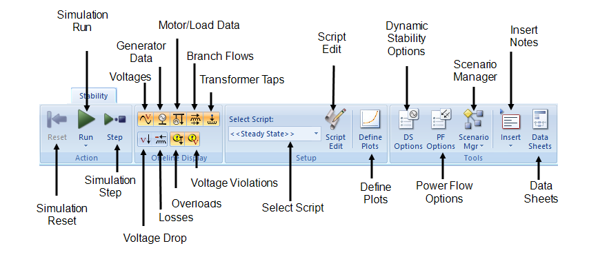
Figure 1: Stability Tab
As you enter the Dynamic Stability focus, EasyPower runs a power flow solution for steady-state—note the power flow results on the one-line.
There are three ways to simulate an event:
- Double-click on an item on the one-line
- Right-click and select from the context menu
- Run a simulation script
A simulation script is a series of commands or instructions for the program to follow. Some scripts have been created in this sample file for you to run.
Note: To perform any command regarding a simulation in the Stability tab, the one-line window needs to be the active window. If the title of the one-line window is not highlighted, click the one-line window once to make it active.
- Click the one-line window to make it active. In the Select Script box in the Stability tab, select the script name ATS on Standby Gen. This script simulates disconnection of some equipment from the utility supply, which results in an ATS transferring connection to a standby generator.
- Click
 Run Simulation.
The one-line shows the power flow results at the end of the simulation. See the figure below. The HV Fuse FS-1 shows the “C>>O” (closed-to-open) symbol next to it, letting us know that the fuse was opened. The ATS has transferred to the generator side.
Click the Plot 2 tab in the DS Plots for DSExample-2.dez window. The plot shows values of voltage, current, and frequency for the standby generator.
To view the spreadsheet data for this plot, you can drag the left edge of the plot area to the right. You can format the plot axes or the plot area by double-clicking on an item.
The DS Messages window at the bottom describes the processes or events that occurred and the time of occurrence.
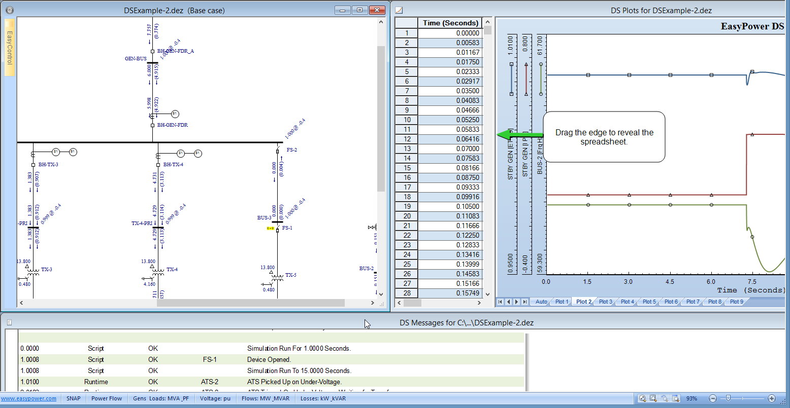
Figure 2: Simulation Results
Simulating a Bus Fault
Double-click on the bus MCC-3 to simulate a bus fault. You can observe the one-line and the message log to view various events that follow the fault. Overcurrent relay R-6 trips to open the breaker BH-TX-3. The contactors for the motors downstream dropout when the voltage on the bus collapses during the fault. The Plot 3 tab in the DS Plots window shows the bus voltage, the current to the faulted bus from the upstream side, and the current contribution from motor M-4.The Autoplot tab shows the voltage and current for the faulted bus.
Dynamic Simulation Options
From the Stability tab that is visible when you select the one-line, click
 DS Options. You can control the simulation through the
Dynamic Stability Options dialog box.
DS Options. You can control the simulation through the
Dynamic Stability Options dialog box.
In the Double-Click Control tab, note the controls for Bus to Fault. The default values are 6 seconds for Simulation End Time and 1 second for Delay Time Length. In the plot from the previous simulation, you will notice that the bus faulted 1 second after the start of the simulation, and the simulation plot ends at 6 seconds. You can control other events in a similar manner.
Simulated Load Shedding
- Select the one-line window and then in the Select Script box, select Load Shedding on Utility Out.
- Click Run Simulation.
This script simulates disconnecting the utility from the rest of the system. When all of the loads are shifted to the generator COGEN, there is a disturbance in various variables. The frequency dips, causing the under-frequency (81) relay R-2 to trip, opening breaker BH-TX-2. After this load trips, the system stabilizes in a few seconds. View Plot 1 and the message log.
Plotting User-Selected Values
When you perform a simulation by double-clicking on the one-line, data is plotted in the AutoPlot tab. Based on the type of simulation, EasyPower chooses which values to display in the AutoPlot. To see values elsewhere in your system, you need to define plots. Nine plots are available with up to a maximum of 5 curves per plot.
Note: AutoPlot results do not appear in simulations run from scripts.
To define a plot:
- Ensure the one-line is selected, and then on the Stability tab, click
 Define Plots.
 - In Plot 4 we will view voltage, current, speed and torque for motor M-2. Select values to plot by choosing the fields for Monitoring, With ID and Next To, as shown in the figure below.
- Click
 Reset Simulation to reset to steady-state prior to running a dynamic simulation again.
 - Click
Run Simulation.
- Click the Plot 4 tab in the DS Plots window to view the effect of utility disconnection and load shedding on motor M-2 values.
Tip: Values can also be selected by first selecting on an open Monitoring cell in the Define Plot window, right-clicking on the motor M-2 on the one-line, and then selecting the desired value type to be plotted.
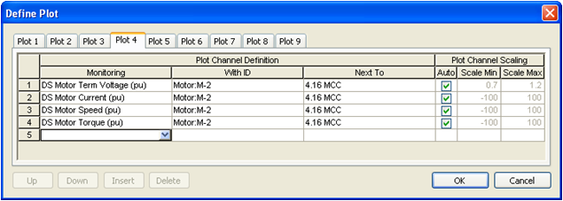
Figure 3: Defining Plots
After the values are entered, close the Define Plot dialog box by clicking OK.
Creating Simulation Scripts
You can write scripts to simulate various events and run them sequentially. Before we run scripts, we need to define plots so that we can view results for the desired values as we just did for motor M-2. Next we will write a script to simulate steady-state for 2 seconds, starting motor M-2, and switching off motor M-1.
- To write a new script, ensure the one-line is selected, and then on the Stability tab, click
 Script Edit. Click
New to add a new script. Type Start M-2 and Stop M-1 as the name of the new script. Add commands to the
script as shown in the figure below. Click
OK in the
Edit Script dialog box and
close in the
Scripts dialog.
Script Edit. Click
New to add a new script. Type Start M-2 and Stop M-1 as the name of the new script. Add commands to the
script as shown in the figure below. Click
OK in the
Edit Script dialog box and
close in the
Scripts dialog.
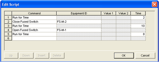
Figure 4: Script Example
- On the Stability tab, in the Select Script box, select the script Start M-2 and Stop M-1.
- Before running a script, it is important to review the initial conditions of the one-line. Since we plan on starting the
motor M-2, the device upstream to this motor needs to be open.
Right-click on the fuse FS-M-2 and select Open and Resolve PF.
- Click
Run Simulation.
- View Plot 4 to see the motor starting values. Browse through other plots to see the effect on other parts of the system.
- To read the values of various variables in the plot, hover the pointer over the plot. The legend shows the values at the pointer positions.
Note: After a script is run, click Reset Simulation to reset to steady state.
Conclusion
This has been a brief tutorial on EasyPower’s Dynamic Stability program. The EasyPower Help topics cover this and other features in greater
depth. To open Help, click  Help in the upper-right corner of the EasyPower window or press F1.
If you have the PowerProtector™ coordination feature, Dynamic Stability can also simulate the response of protective devices. You can simulate contactors dropping out from excessive voltage drop, or an ATS switching to emergency power. Remember to enter data in the Database Edit focus on the Stability tab of various equipment data dialogs first. Make use of scripts to simulate sequential events and use the Define Plots feature to monitor values.